stable/docs/freqai-outlier-detection.md

Outlier detection

Equity and crypto markets suffer from a high level of non-patterned noise in the form of outlier data points. FreqAI implements a variety of methods to identify such outliers and hence mitigate risk.

Identifying outliers with the Dissimilarity Index (DI)

The Dissimilarity Index (DI) aims to quantify the uncertainty associated with each prediction made by the model.

The user can tell FreqAI to remove outlier data points from the training/test data sets using the DI by including the following statement in the config:

    "freqai": {
        "feature_parameters" : {
            "DI_threshold": 1
        }
    }

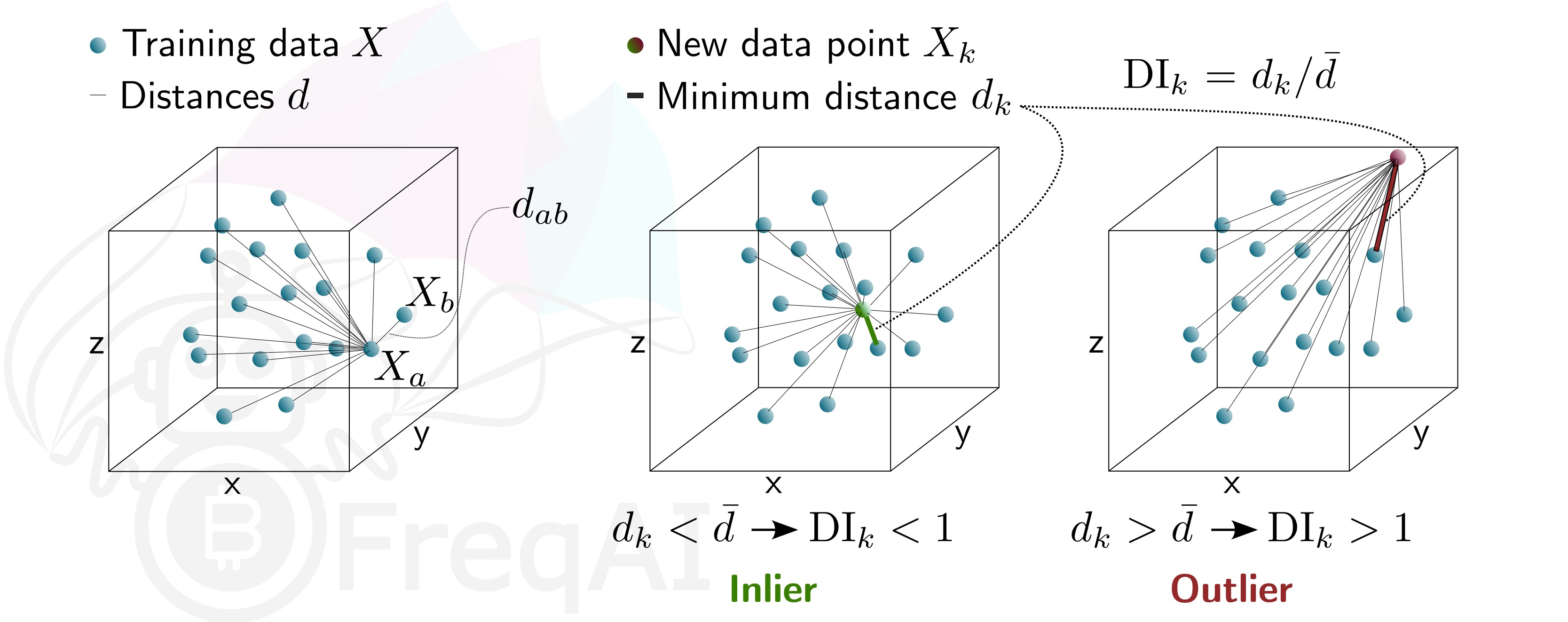
The DI allows predictions which are outliers (not existent in the model feature space) to be thrown out due to low levels of certainty. To do so, FreqAI measures the distance between each training data point (feature vector), X_{a}, and all other training data points:

 d_{ab} = \sqrt{\sum_{j=1}^p(X_{a,j}-X_{b,j})^2} 

where d_{ab} is the distance between the normalized points a and b, and p is the number of features, i.e., the length of the vector X. The characteristic distance, \overline{d}, for a set of training data points is simply the mean of the average distances:

 \overline{d} = \sum_{a=1}^n(\sum_{b=1}^n(d_{ab}/n)/n) 

\overline{d} quantifies the spread of the training data, which is compared to the distance between a new prediction feature vectors, X_k and all the training data:

 d_k = \arg \min d_{k,i} 

This enables the estimation of the Dissimilarity Index as:

 DI_k = d_k/\overline{d} 

The user can tweak the DI through the DI_threshold to increase or decrease the extrapolation of the trained model. A higher DI_threshold means that the DI is more lenient and allows predictions further away from the training data to be used whilst a lower DI_threshold has the opposite effect and hence discards more predictions.

Below is a figure that describes the DI for a 3D data set.

Identifying outliers using a Support Vector Machine (SVM)

The user can tell FreqAI to remove outlier data points from the training/test data sets using a Support Vector Machine (SVM) by including the following statement in the config:

    "freqai": {
        "feature_parameters" : {
            "use_SVM_to_remove_outliers": true
        }
    }

The SVM will be trained on the training data and any data point that the SVM deems to be beyond the feature space will be removed.

FreqAI uses sklearn.linear_model.SGDOneClassSVM (details are available on scikit-learn's webpage here (external website)) and the user can elect to provide additional parameters for the SVM, such as shuffle, and nu.

The parameter shuffle is by default set to False to ensure consistent results. If it is set to True, running the SVM multiple times on the same data set might result in different outcomes due to max_iter being to low for the algorithm to reach the demanded tol. Increasing max_iter solves this issue but causes the procedure to take longer time.

The parameter nu, very broadly, is the amount of data points that should be considered outliers and should be between 0 and 1.

Identifying outliers with DBSCAN

The user can configure FreqAI to use DBSCAN to cluster and remove outliers from the training/test data set or incoming outliers from predictions, by activating use_DBSCAN_to_remove_outliers in the config:

    "freqai": {
        "feature_parameters" : {
            "use_DBSCAN_to_remove_outliers": true
        }
    }

DBSCAN is an unsupervised machine learning algorithm that clusters data without needing to know how many clusters there should be.

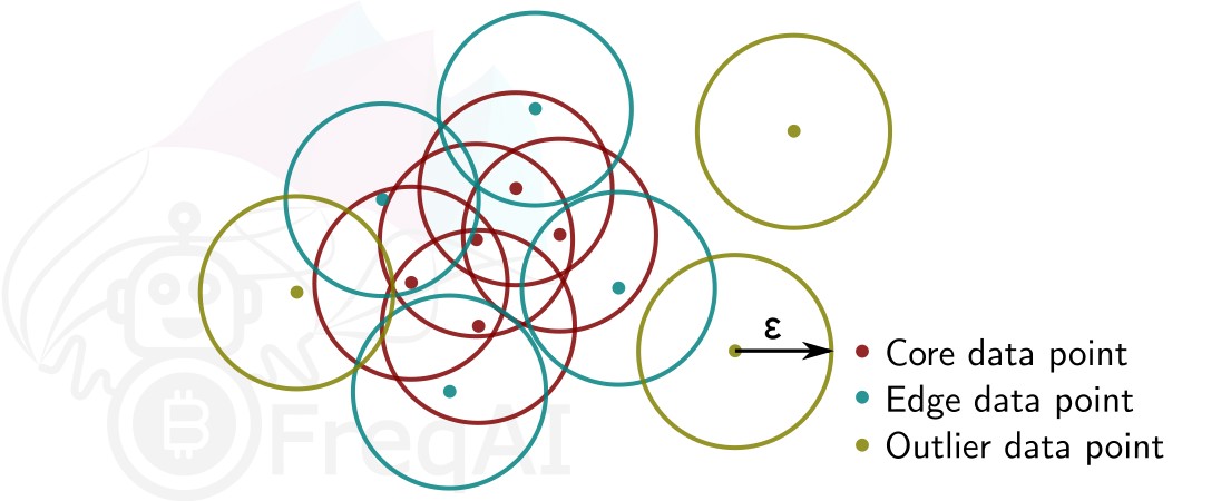
Given a number of data points N, and a distance \varepsilon, DBSCAN clusters the data set by setting all data points that have N-1 other data points within a distance of \varepsilon as core points. A data point that is within a distance of \varepsilon from a core point but that does not have N-1 other data points within a distance of \varepsilon from itself is considered an edge point. A cluster is then the collection of core points and edge points. Data points that have no other data points at a distance <\varepsilon are considered outliers. The figure below shows a cluster with N = 3.

FreqAI uses sklearn.cluster.DBSCAN (details are available on scikit-learn's webpage here (external website)) with min_samples (N) taken as 1/4 of the no. of time points in the feature set. eps (\varepsilon) is computed automatically as the elbow point in the k-distance graph computed from the nearest neighbors in the pairwise distances of all data points in the feature set.